6 views
Excel Hacks: Pivot Table

What is a Pivot Table?
A Pivot Table is used to summarise, sort, reorganize, group, count, total or average data stored in a table. It allows us to transform columns into rows and rows into columns. It allows grouping by any field (column) and using advanced calculations on them.
How to create a Pivot Table?
Step 1: Click a cell in the source data or table range. ( There should be some data).
Step 2: Go to the insert tab and click on Pivot Table.
Step 3: A dialogue box will open with the name Create Pivot Table.
Step 4: Choose where you want the Pivot Table report to be placed: New worksheet or Existing worksheet. Choosing a new worksheet is more convenient but if you want to insert Pivot Table in the same worksheet you can go for an existing worksheet. Then click ok.
Shortcut to insert Pivot Table: Alt+N+V
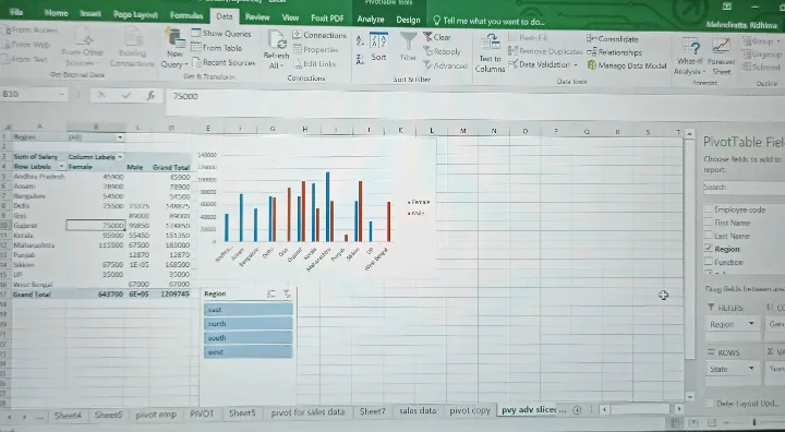
After clicking ok on the dialogue box a Pivot Table gets inserted along with a Pivot table editor box named as Pivot Table fields. With the help of the Pivot table editor, you can analyse your data in numerous ways. It gives 4 options for data analysis:
1. Filters
2. Columns
3. Rows
4. Values
As in the beginning, I wrote that with the help of the Pivot Table you can convert rows into columns and columns into rows. It can happen through this editor only.
When to use Pivot Table?
You will derive the best use of Pivot Table when you have tabular data and want to analyse such data in as much detail as possible. Because Pivot Table opens you to different ways of advanced analysis such as using slicers and inserting pivot charts. Charts are more catchy and give a bird's eye view of the data in a glimpse. So try this feature now and explore what more it can do for you.
A Pivot Table is used to summarise, sort, reorganize, group, count, total or average data stored in a table. It allows us to transform columns into rows and rows into columns. It allows grouping by any field (column) and using advanced calculations on them.
How to create a Pivot Table?
Step 1: Click a cell in the source data or table range. ( There should be some data).
Step 2: Go to the insert tab and click on Pivot Table.
Step 3: A dialogue box will open with the name Create Pivot Table.
Step 4: Choose where you want the Pivot Table report to be placed: New worksheet or Existing worksheet. Choosing a new worksheet is more convenient but if you want to insert Pivot Table in the same worksheet you can go for an existing worksheet. Then click ok.
Shortcut to insert Pivot Table: Alt+N+V
After clicking ok on the dialogue box a Pivot Table gets inserted along with a Pivot table editor box named as Pivot Table fields. With the help of the Pivot table editor, you can analyse your data in numerous ways. It gives 4 options for data analysis:
1. Filters
2. Columns
3. Rows
4. Values
As in the beginning, I wrote that with the help of the Pivot Table you can convert rows into columns and columns into rows. It can happen through this editor only.
When to use Pivot Table?
You will derive the best use of Pivot Table when you have tabular data and want to analyse such data in as much detail as possible. Because Pivot Table opens you to different ways of advanced analysis such as using slicers and inserting pivot charts. Charts are more catchy and give a bird's eye view of the data in a glimpse. So try this feature now and explore what more it can do for you.